This is the first in a series of posts describing the functions and algorithms that I have implemented in the R package bayesImageS.

Gibbs sampling was originally designed by Geman & Geman (1984) for drawing updates from the Gibbs distribution, hence the name. However, single-site Gibbs sampling exhibits poor mixing due to the posterior correlation between the pixel labels. Thus it is very slow to converge when the correlation (controlled by the inverse temperature \(\beta\)) is high.

The algorithm of Swendsen & Wang (1987) addresses this problem by forming clusters of neighbouring pixels, then updating all of the labels within a cluster to the same value. When simulating from the prior, such as a Potts model without an external field, this algorithm is very efficient.

---

The SW function in the PottsUtils package is implemented in a combination of R and C. The swNoData function in bayesImageS is implemented using RcppArmadillo, which gives it a speed advantage. It is worth noting that the intention of bayesImageS is not to replace PottsUtils. Rather, an efficient Swendsen-Wang algorithm is used as a building block for implementations of ABC (Grelaud et al., 2009), path sampling (Gelman & Meng, 1998), and the exchange algorithm (Murray et al., 2006). These other algorithms will be covered in future posts.

There are two things that we want to keep track of in this simulation study: the speed of the algorithm and the distribution of the summary statistic. We will be using system.time(..) to measure both CPU and elapsed (wall clock) time taken for the same number of iterations, for a range of inverse temperatures:

beta <- seq(0,2,by=0.1)
tmMx.PU <- tmMx.bIS <- matrix(nrow=length(beta),ncol=2)
rownames(tmMx.PU) <- rownames(tmMx.bIS) <- beta
colnames(tmMx.PU) <- colnames(tmMx.bIS) <- c("user","elapsed")

We will discard the first 100 iterations as burn-in and keep the remaining 500.

iter <- 600
burn <- 100
samp.PU <- samp.bIS <- matrix(nrow=length(beta),ncol=iter-burn)

The distribution of pixel labels can be summarised by the sufficient statistic of the Potts model:

\[ S(z) = \sum_{i \sim \ell \in \mathscr{N}} \delta(z_i, z_\ell) \]

where \(i \sim \ell \in \mathscr{N}\) are all of the pairs of neighbours in the lattice (ie. the cliques) and \(\delta(u,v)\) is 1 if \(u = v\) and 0 otherwise (the Kronecker delta function). swNoData returns this automatically, but with SW we will need to use the function sufficientStat to calculate the sufficient statistic for the labels.

library(bayesImageS)
library(PottsUtils)

## 
## Attaching package: 'PottsUtils'

## The following objects are masked from 'package:bayesImageS':
## 
##     getBlocks, getEdges, getNeighbors

mask <- matrix(1,50,50)
neigh <- getNeighbors(mask, c(2,2,0,0))
block <- getBlocks(mask, 2)
edges <- getEdges(mask, c(2,2,0,0))

n <- sum(mask)
k <- 2
bcrit <- log(1 + sqrt(k))
maxSS <- nrow(edges)

for (i in 1:length(beta)) {
  # PottsUtils
  tm <- system.time(result <- SW(iter,n,k,edges,beta=beta[i]))
  tmMx.PU[i,"user"] <- tm["user.self"]
  tmMx.PU[i,"elapsed"] <- tm["elapsed"]
  res <- sufficientStat(result, neigh, block, k)
  samp.PU[i,] <- res$sum[(burn+1):iter]
  print(paste("PottsUtils::SW",beta[i],tm["elapsed"],median(samp.PU[i,])))
  
  # bayesImageS
  tm <- system.time(result <- swNoData(beta[i],k,neigh,block,iter))
  tmMx.bIS[i,"user"] <- tm["user.self"]
  tmMx.bIS[i,"elapsed"] <- tm["elapsed"]
  samp.bIS[i,] <- result$sum[(burn+1):iter]
  print(paste("bayesImageS::swNoData",beta[i],tm["elapsed"],median(samp.bIS[i,])))
}

## [1] "PottsUtils::SW 0 4.714 2454"
## [1] "bayesImageS::swNoData 0 0.194 2450"
## [1] "PottsUtils::SW 0.1 2.834 2576"
## [1] "bayesImageS::swNoData 0.1 0.239000000000001 2575"
## [1] "PottsUtils::SW 0.2 2.676 2697"
## [1] "bayesImageS::swNoData 0.2 0.250999999999999 2699"
## [1] "PottsUtils::SW 0.3 2.695 2830.5"
## [1] "bayesImageS::swNoData 0.3 0.262999999999998 2834.5"
## [1] "PottsUtils::SW 0.4 2.536 2972"
## [1] "bayesImageS::swNoData 0.4 0.312000000000001 2977"
## [1] "PottsUtils::SW 0.5 2.348 3131"
## [1] "bayesImageS::swNoData 0.5 0.277000000000001 3133"
## [1] "PottsUtils::SW 0.6 2.47 3310"
## [1] "bayesImageS::swNoData 0.6 0.277000000000001 3303"
## [1] "PottsUtils::SW 0.7 2.136 3516.5"
## [1] "bayesImageS::swNoData 0.7 0.268000000000001 3520.5"
## [1] "PottsUtils::SW 0.8 2.172 3775.5"
## [1] "bayesImageS::swNoData 0.8 0.263000000000002 3776"
## [1] "PottsUtils::SW 0.9 1.932 4167"
## [1] "bayesImageS::swNoData 0.9 0.244000000000003 4188"
## [1] "PottsUtils::SW 1 1.714 4527"
## [1] "bayesImageS::swNoData 1 0.234999999999999 4526.5"
## [1] "PottsUtils::SW 1.1 1.69 4680"
## [1] "bayesImageS::swNoData 1.1 0.228999999999999 4674"
## [1] "PottsUtils::SW 1.2 1.643 4756"
## [1] "bayesImageS::swNoData 1.2 0.225999999999999 4759"
## [1] "PottsUtils::SW 1.3 1.618 4812"
## [1] "bayesImageS::swNoData 1.3 0.224000000000004 4811"
## [1] "PottsUtils::SW 1.4 1.635 4846"
## [1] "bayesImageS::swNoData 1.4 0.221000000000004 4843"
## [1] "PottsUtils::SW 1.5 1.674 4864"
## [1] "bayesImageS::swNoData 1.5 0.235999999999997 4863"
## [1] "PottsUtils::SW 1.6 1.707 4875"
## [1] "bayesImageS::swNoData 1.6 0.216999999999999 4875"
## [1] "PottsUtils::SW 1.7 1.603 4883"
## [1] "bayesImageS::swNoData 1.7 0.213000000000001 4885"
## [1] "PottsUtils::SW 1.8 1.741 4890"
## [1] "bayesImageS::swNoData 1.8 0.216999999999999 4889"
## [1] "PottsUtils::SW 1.9 1.672 4893"
## [1] "bayesImageS::swNoData 1.9 0.219000000000001 4893"
## [1] "PottsUtils::SW 2 1.622 4896"
## [1] "bayesImageS::swNoData 2 0.210999999999999 4896"

Here is the comparison of elapsed times between the two algorithms (in seconds):

summary(tmMx.PU)

##       user          elapsed     
##  Min.   :1.879   Min.   :1.603  
##  1st Qu.:1.980   1st Qu.:1.672  
##  Median :2.143   Median :1.741  
##  Mean   :2.448   Mean   :2.135  
##  3rd Qu.:2.787   3rd Qu.:2.470  
##  Max.   :4.624   Max.   :4.714

summary(tmMx.bIS)

##       user           elapsed      
##  Min.   :0.7030   Min.   :0.1940  
##  1st Qu.:0.7830   1st Qu.:0.2190  
##  Median :0.8330   Median :0.2350  
##  Mean   :0.8634   Mean   :0.2398  
##  3rd Qu.:0.9740   3rd Qu.:0.2630  
##  Max.   :1.0530   Max.   :0.3120

boxplot(tmMx.PU[,"elapsed"],tmMx.bIS[,"elapsed"],ylab="seconds elapsed",names=c("SW","swNoData"))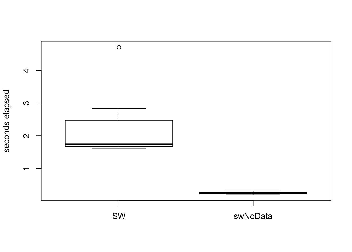

On average, swNoData using RcppArmadillo is seven times faster than SW.

library(lattice)
s_z <- c(samp.PU,samp.bIS)
s_x <- rep(beta,times=iter-burn)
s_a <- rep(1:2,each=length(beta)*(iter-burn))
s.frame <- data.frame(s_z,c(s_x,s_x),s_a)
names(s.frame) <- c("stat","beta","alg")
s.frame$alg <- factor(s_a,labels=c("SW","swNoData"))
xyplot(stat ~ beta | alg, data=s.frame)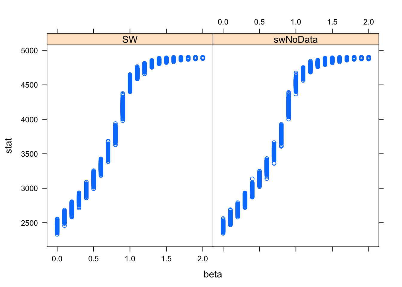

plot(c(s_x,s_x),s_z,pch=s_a,xlab=expression(beta),ylab=expression(S(z)))
abline(v=bcrit,col="red")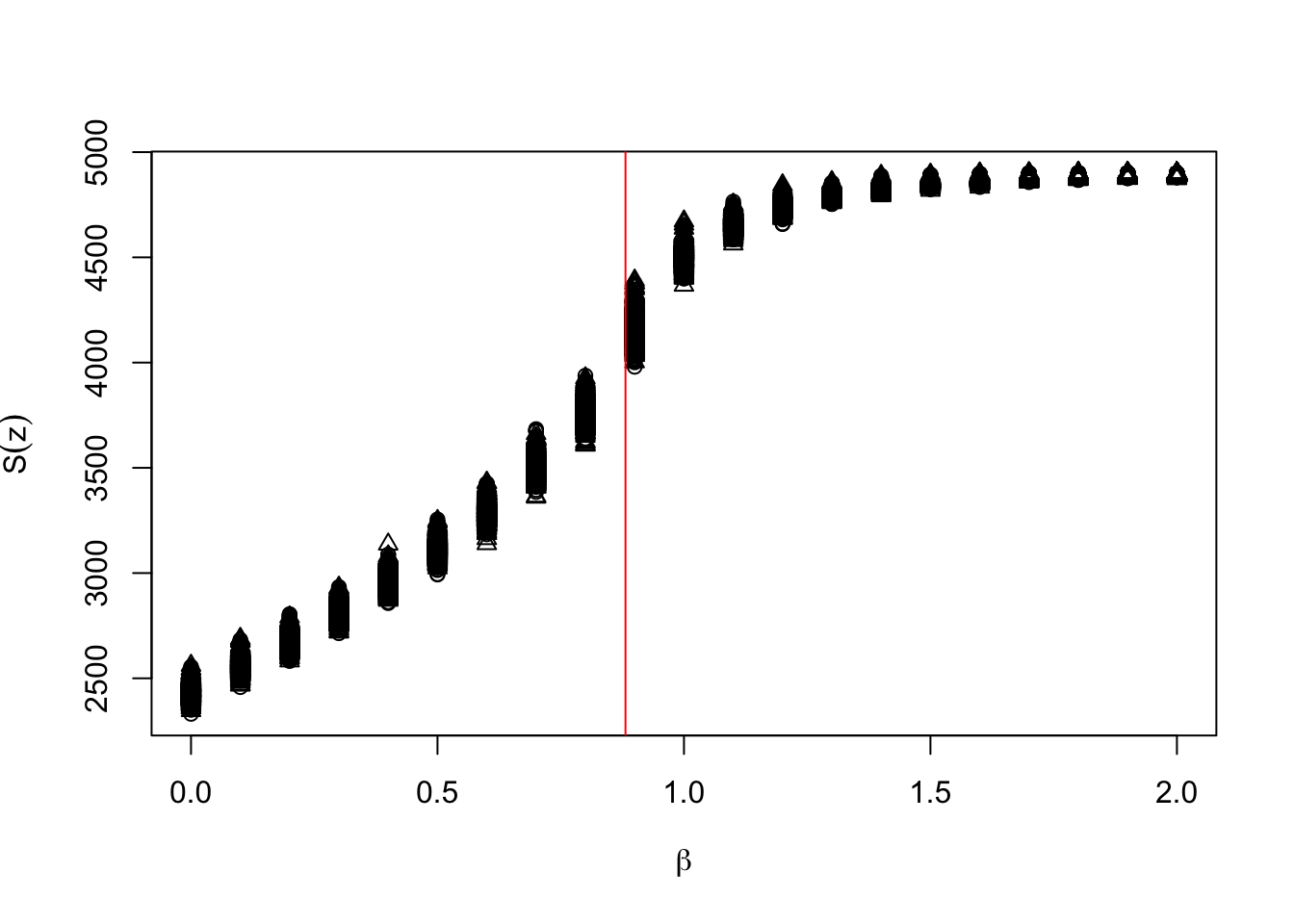

The overlap between the two distributions is almost complete, although it is a bit tricky to verify that statistically. The relationship between \(beta\) and \(S(z)\) is nonlinear and heteroskedastic.

rowMeans(samp.bIS) - rowMeans(samp.PU)

##  [1] -0.772 -0.590 -1.054  2.712  4.582 -0.066 -8.166  0.706 -4.264 16.750
## [11] -1.108 -3.054  4.052 -0.070 -2.302 -0.448 -0.266  0.334 -1.012 -0.664
## [21]  0.406

apply(samp.PU, 1, sd)

##  [1] 34.630195 33.934640 35.704262 35.545965 37.622211 42.116290 42.019891
##  [8] 50.341777 54.788287 68.669494 45.133021 31.436476 26.122016 19.637341
## [15] 14.993307 13.045745 10.683573  7.688128  6.308355  5.076720  4.626509

apply(samp.bIS, 1, sd)

##  [1] 33.482151 35.825568 35.264450 38.432163 41.293441 39.750721 43.299385
##  [8] 48.546938 51.764641 65.954575 43.853962 31.313644 25.747320 18.276720
## [15] 16.313447 11.935447 10.038472  7.979904  6.436971  5.363614  4.687996

s.frame$beta <- factor(c(s_x,s_x))
s.fit <- aov(stat ~ alg + beta, data=s.frame)
summary(s.fit)

##                Df    Sum Sq   Mean Sq   F value Pr(>F)    
## alg             1 3.880e+02       388 3.310e-01  0.565    
## beta           20 1.743e+10 871316719 7.431e+05 <2e-16 ***
## Residuals   20978 2.460e+07      1173                     
## ---
## Signif. codes:  0 '***' 0.001 '**' 0.01 '*' 0.05 '.' 0.1 ' ' 1

TukeyHSD(s.fit,which="alg")

##   Tukey multiple comparisons of means
##     95% family-wise confidence level
## 
## Fit: aov(formula = stat ~ alg + beta, data = s.frame)
## 
## $alg
##                  diff        lwr      upr     p adj
## swNoData-SW 0.2717143 -0.6546239 1.198052 0.5653439

References

Gelman, A. & Meng, X-L (1998) Simulating normalizing constants: from importance sampling to bridge sampling to path sampling

Geman, S. and Geman, D. (1984) Stochastic relaxation, Gibbs distributions and the Bayesian restoration of images

Grelaud, A., Robert, C.P., Marin, J-M, Rodolphe, F. & Taly, J-F (2009) ABC likelihood-free methods for model choice in Gibbs random fields

Murray, I., Ghahramani, Z. & MacKay, D.J.C. (2006) MCMC for Doubly-intractable Distributions

Swendsen, R.H. & Wang, J-S (1987) Nonuniversal critical dynamics in Monte Carlo simulations